We were making a training at work about ensemble models. When we were discussing different techniques like bagging, boosting, and stacking, we also came on the subject of gradient boosting. Intuitively, gradient boosting, by training on the residuals made sense. However, the name gradient boosting did not right away. This post we are exploring the name of gradient boosting and of course also the model itself.
Intuition
Single decision tree
Gradient boosting is often used as an optimization technique for decision trees. Decision trees are rule-based models. Using a single decision tree often leads to models with high variance, i.e. overfitting. Below we can see why this happens.

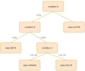
50% split at every node
You can imagine a tree, where at every node approximately 50% of the data is being split. The nodes that are deep in the tree, will only see a small subset of the data and make splits on these small subsets. The chances that these subsets don’t represent the real distribution of the data increase by depth, and so does the chance of overfitting. Another limitation of decision trees is that they do not optimize an overall loss function. Decision trees are trained ‘greedy’, which means that they minimize loss at every node. However, minimizing loss at a node level does not guarantee a minimal loss at a tree level.
Gradient boosting trees
Gradient boosting trees solves part of the limitation mentioned above. Instead of training a single tree, multiple trees are trained sequentially. To lower the variance of the trees, they are however restricted. They are turned into weak learners by setting limits on the depth of the trees. The decision trees depth if often chosen between 3 and 6 layers. We allow a little bit of depth so that we can compare jointly occurring of variables. If a tree has a depth of three layers, we can compare conditions like this:
if A and B and C then;
Okay, now we have talked about the limitation of decision trees, let’s look how gradient boosting uses trees and tries to overcome these problems. Note that we will focus this entire post on regression problems and therefore assume numerical data, not categorical.
Gradient boosting trees is recurrently defined as a set of MM trees
Fm(x)=Fm−1(x)+hm(x)Fm(x)=Fm−1(x)+hm(x)
Fm(x)Fm(x) is an iterative boost of the model, by adding a decision tree hm(x)hm(x) to previous iteration of the model Fm−1(x)Fm−1(x). The tree hm(x)hm(x) is trained on the residuals of Fm−1(x)Fm−1(x). Residuals are the difference with the true labels yy and the predictions of the model ^yy^.
hm(x)=y−Fm−1(x)hm(x)=y−Fm−1(x)
Intuitively this makes a lot of sense. We missed a few spots in our previous model Fm−1(x)Fm−1(x) and therefore we let the next model hm(x)hm(x) focus on those spots. And by iterating a few times, we will approach closer to yy until convergence.
It also takes into account the problems we saw at a single decision tree.
- Greedy learning, no overall loss function is optimized.
- Decisions are made on small subsets of the data.
The overall loss is now minimized, but we’ll get to proof of that later! The decisions are now not made on small subsets, because we don’t let the trees get too deep and every iteration a new tree is trained on all the data (now being residuals). Every new tree trains actually on new rescaled data. The new tree will focus on the samples where the previous iteration Fm−1Fm−1 is very wrong as this leads to large residuals. Every new tree focuses on the errors of the previous one, by taking into account all the data, and not a subset of the data! This distinction is very important as this reduces the chance of overfitting a lot.
Interested in reading the whole blog? Check out Ritchie’s website.


