Ritchie is a Data Scientist & Big Data Engineer at Xomnia. Besides working at Xomnia, he writes blogs on his website about all kinds of machine- and deep learning topics, such as: “Computer build me a bridge” and “Programming a neural network from scratch”. Expect more interesting blogs from Ritchie in the future.
The Opportunity
For a project at Xomnia, I had the opportunity to do a cool computer vision assignment. We tried to predict the input of a road safety model. Eurorap is such a model. In short, it works something like this. You deploy some cars, mount cameras on them, and drive around on the road you’re interested in inspecting. The ‘Google Streetview’ like material you’ve collected is sent to a crowdsourced workforce (at Amazon they are called Mechanical Turks) to manually label the footage.

Manually labeling of pictures is, of course, a very time consuming, costly, not scalable, and last but not least boooring task!
Just imagine yourself clicking through thousands of images like the one shown below.

This post describes the proof of concept we’ve done, and how we’ve implemented it in Pytorch.
Dataset
The taped video material is cut into images that are shot every 10 meters. Even a Mechanical Turk has trouble not shooting itself of boredom when he has to fill in 300 labels of what he sees every 10 meters. To make the work a little bit more pleasant he now only has to fill in the labels every 100 meters for what they had seen in the 10 pictures. However, this method has led to the terrible labeling of footage. Every object that you drive by within these 100 meters is labeled to all 10 images, whilst most of the time it is only visible in 2~4 images!
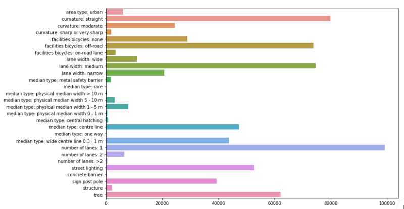
We made a proof of concept and we’ve only regarded a small subset of all labels. In total there are approximately 300. We based our analysis on 28 labels. Also, because of the problem of the mislabeled objects, we’ve mostly chosen labels that are visible and parallel to the road. These labels seem likely to hold true for all the 10 images. For instance, a road that has an emergency lane in one image is likely to have an emergency lane in the following images.
Below you’ll see a plot with the labels we have trained our model on, and the number of occurrences of that specific label. In total, approximately 100,000 images were in our dataset.

Transfer learning
There is a reasonable amount of images to work with, however, the large imbalances in the labels, the errors in labeling, and the amount of data required for the data-hungry models (called neural networks) make it unlikely that we have enough data to properly train a robust computer vision model.
To give you an idea of the scale of data used in this model compared to other projects. The record-breaking convolutional neural networks you read about in the news are often trained on the imageNet dataset, which contains 1.2 million images. These modern ConvNets (convolutional neural networks) are trained for ~2 weeks on heavy duty GPU’s to go from their random initialization of weights, to achieve a configuration that is able to win prices.
It would be nice if we don’t have to waste all this computational effort and somehow could transfer what we have learned in one problem (imageNet) to another (roadImages). Luckily, with ConvNets this isn’t a bad idea and there is quite some logical intuition in doing so. Neural networks are often regarded as black box classifiers. And for the classification part, this is currently somewhat true. But for traditional ConvNet, architectures there is a clear distinction between the classification and the feature extraction.
And this feature extraction part is:
- Not so black box at all.
- Very transferable.
Not so black box at all
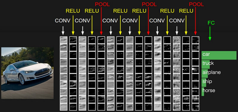
When taking a look at which pixels of an image result in activations (i.e. neurons having a large output) in convolutional layers, we can get some intuition on what is happening and meant with feature extraction.

When we look at the activated neurons in the first layers, we can clearly identify the car. This means that there are a lot of low-level features activated. Even so much that we can still identify the car by the activated neurons. The lower level features are, for instance, edges, shadows, textures, lines, colors, etc.

Based on the activation of lower features, new neurons will activate, growing in hierarchy and complexity. Activated edges combine in the activations of curves, which can lead to the activation of objects in combination with other features, objects like a tire or a grill. Let’s say that in the image above a neuron is highly activated because of a complex feature like a car grill. We wouldn’t be able to see this in an image of the activations. As there is only one grill on the car (and one grill detector in our network), we would only see one activated neuron, i.e. one white pixel!

Very transferable
Along this line of thought, it seems pretty reasonable to assume that these lower level features extend to more than just cars. Almost every picture has got edges, shadows, colors and so forth. This means that a lot of the weights in the feature extraction neurons within a price winning ConvNet are set just right, or at least very close to our configuration goal of the weights.
This works so well, that we can pre-train a ConvNet on a large dataset like ImageNet and transfer the ConvNet to a problem with a relatively small dataset (that normally would be insufficient for this ConvNet architecture). The pre-trained model still needs to be fine-tuned. There are a few options like freezing the lower layers and retraining the upper layers with a lower learning rate, fine-tuning the whole net, or retraining the classifier.
In our case, we fine-tuned the feature extraction layers with low learning rates and changed the classifier of the model.
Implementation, Results & Conclusion
If you are interested in reading the full blog, visit Ritchie’s website to read the implementation process, the exciting results and the conclusion.


